CS 5043: HW3: Convolutional Neural Networks

Objectives

Implement general code that constructs Convolutional Neural Network models based on a set of parameters.
Identify two model configurations that perform reasonably well on the validation set.
Perform a full set of 5 rotations to demonstrate consistency in the model performance.

Assignment Notes

Deadline: Tuesday, March 12th @11:59pm.
Hand-in procedure: submit to a zip file to the HW3 dropbox on Gradescope (details below)
This work is to be done on your own. While general discussion about Python, TensorFlow and Keras is okay, sharing solution-specific code is inappropriate. Likewise, you may not download code solutions to this problem from the network or a LLM.
All code that we release for the class may be used.
Do not submit MSWord documents.

Data Set

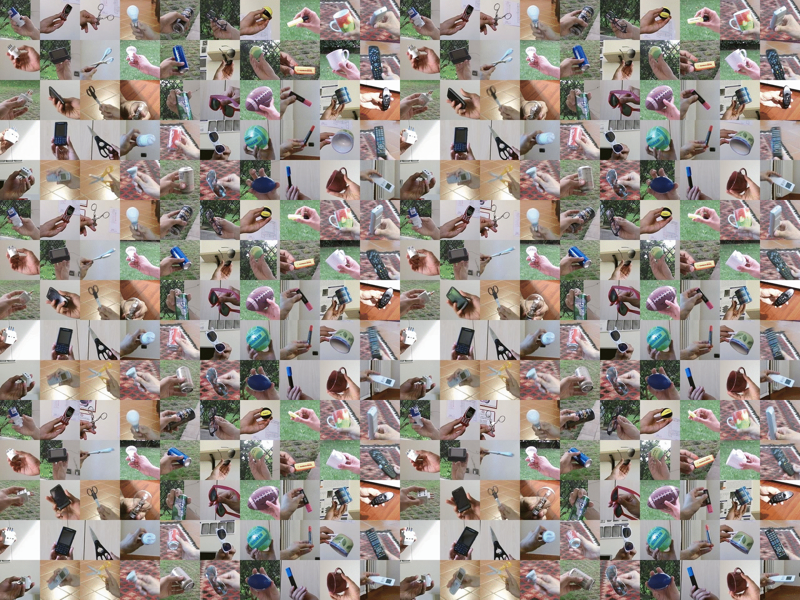
The Core50 data set is a large database of videos of objects as they are being moved/rotated under a variety of different lighting and background conditions. Our general task is to classify the object being shown in a single frame of one of these videos.

Data Organization

A subset of the database is available on OSCER: /home/fagg/datasets/core50/core50_128x128
Two zip files are also downloadable from /home/fagg/datasets/core50
- core50_hw3_full.zip: the full dataset for HW3 (this is really large)
- core50_hw3_mini.zip: conditions s1, s2 and s3. This is a subset of the full dataset and is more feasible for download to your own personal machine. Note that if you are using this dataset, you will need to make changes to your load_data_set() function.
The database is partitioned into different conditions (s1, s2, ...). These conditions represent different backgrounds
Within the condition, you will find individual objects contained in their own directories. Objects 1...5 are of the same class (plug adapters); objects 6...10 are the same class (mobile phone), etc.
Within each object directory is a sequence of PNG files. The last number of the file name is the image sequence number
Each image is 128 x 128 in size and is color (Red, Green, Blue channels)
A metadata file (core50_df.pkl) contains information about all files in the dataset and their class labels. Specifically, it contains one DataFrame that describes each image in the dataset. Specifically, each row contains:
- condition: int index of the background condition (1...12)
- object: unique object identifier
- fname: name of the file relative to the main dataset directory
- class: object class (0...9)
- example: index of object within its class (0...4)
- problem_class: initialized to the empty string
Provided code will parse this metadata file and create training/validation/testing sets for you.
A pre-constructed set of data folds exist in two subdirectories: datasets_by_fold_10_objects and datasets_by_fold_4_objects. We will use the latter for this assignment.
A copy of the key parts of the pre-constructed datasets is currently stored in /scratch/fagg/core50. Access to this copy is faster than the original one (but will only last so long).

Provided Code

We are providing the following code posted on the main course web page:

hw3_base.py: An experiment-execution module. Parameter organization, loading data, executing experiment, saving results.
hw3_parser.py: An argument parser.
core50.py: A class that will translate the metadata file into TF Datasets for the training, validation and testing sets.
hw3.sh: A sample batch file
exp.txt, oscer.txt, and net_shallow.txt: command line parameter files that are a starting point for your work
job_control.py was provided in a previous assignment

Prediction Problem

We will focus on classifying one of four object classes: plug adapter, mobile phone, glass, remote control. For HW 3, each fold will contain one instance of each of the object classes. We will use three folds for training, one for validation and one for testing. Hence, we constructing models that are intended to work for any previously unseen instance of an object class.

Architectures

You will create two convolutional neural networks to distinguish these four classes: one will be a shallow network and the other will be a deep network. The shallow network should only be composed of a few layers. Each architecture will nominally have the following structure:

One or more convolutional filters, each (possibly) followed by a max pooling layer.
- Use your favorite activation function
- In most cases, each conv/pooling layer will involve some degree of size reduction (striding)
- Convolutional filters should not be larger than 7x7 (as the size of the filter gets larger, the memory requirements explode for training)
GlobalMaxPool
One or more dense layers
- Choose your favorite activation function
One output layer with four units (one for each class). The activation for this layer should be softmax
Loss: sparse categorical cross-entropy. The data set contains a scalar desired output that is an integer class index (0,1,2,3). The sparse automatically translates this into a 1-hot encoded desired output.
Additional metric: sparse categorical accuracy

Since the data set is relatively small (in terms of the number of distinct objects), it is important to take steps to address the over-fitting problem. Here are the key tools that you have:

L1 or L2 regularization
Dropout. Only use dropout with Dense layers
Sparse Dropout. Only use sparse dropout only with Convolutional layers
Try to keep the number of trainable parameters small (no more than one million)

Experiments

The primary objective is to get your model building code working properly and to execute some simple experiments.
Spend a little time informally narrowing down the details of your two architectures, including the hyper-parameters (layer sizes, dropout, regularization). Don't spend a lot of time on this step
Once you have made your choice of architecture for each, you will perform five rotation for each model (so, a total of 10 independent runs)
Figure 1 and 2: Learning curves (validation accuracy and loss as a function of epoch) for the shallow and deep models. Put all five curves on a single plot.
Figure 3: Generate a histogram of test set accuracy (a total of 10 samples). The shallow and deep samples should have different colors (an alpha of 0.5 will give the histogram values some transparency).
Figure 4: For a small sample of test set images, show each image and the output probability distribution from your two models. The probability distribution should be written on top of the example image.
Figures 5a...j: Create one confusion matrix for each of the test sets (so, a total of 10 figures). Scikit-Learn's Confusion Matrix Implementation

Hints / Notes

Start small: get the pipeline working first on a small network.
We use a general function for creating networks that takes as input a set of parameters that define the configuration of the convolutional layers and dense layers. By changing these parameters, we can even change the number of layers. This makes it much easier to try a variety of things without having to re-implement or copy a lot of code.
Remember to check your model summary to make sure that it matches your expectations
Cache your datasets to RAM (Use "" for the --cache argument).
Before performing a full execution on the supercomputer, look carefully at your memory usage (our big model + caching requires 30-40GB of memory)
CPUS_PER_TASK in the batch file and at the command line should be about 64
Adjust your batch size so you almost fill up your VRAM.

You can access the numpy arrays that a TF Dataset generates using something like this:

       for in, out in ds.take(1):
          # in and out are numpy arrays.  For our case,
          #   in.shape is (batch_size, 128, 128, 3)
          #   out.shape is (batch_size,)

ds.take() produces a new dataset that has only the first batch in ds.

What to Hand In

A single zip file that contains:

All of your python code, including your network building code
Your batch file(s)
One sample stdout file
A report:
- If your visualization code is a Jupyter Notebook, then turn it in
- Otherwise, turn in a pdf file
The report will include:
- Your figures
- A written reflection that answers the following questions:
  - How many parameters were needed by your shallow and deep networks?
  - What can you conclude from the validation accuracy learning curves for each of the shallow and deep networks? How confident are you that you have created models that you can trust?
  - Did your shallow or deep network perform better with respect to the test set? (no need for a statistical argument here)

Grading

20 pts: Clean code for model building (including documentation)
10 pts: Figure 1: Shallow/deep loss learning curves
10 pts: Figure 2: Shallow/deep accuracy learning curves
15 pts: Figure 3: Test set histograms
15 pts: Figure 4: Images + probability distributions
10 pts: Figure 5: Confusion matrices
20 pts: Reflection

andrewhfagg -- gmail.com

Last modified: Mon Mar 4 12:19:56 2024